XLOOKUP is the new kid on the block for lookup functions in Microsoft Excel. It was first introduced back in 2019 as part of Microsoft 365 and was billed as the successor to VLOOKUP and/or HLOOKUP. Whilst many Excel users are staying loyal to VLOOKUP, it is more than worthwhile to take a look at the capabilities of using the XLOOKUP function.
XLOOKUP offers significant advantages over its predecessors. XLOOKUP allows for searches in any direction within your data range, not just vertically or horizontally, providing greater flexibility in how you set out your data. It easily handles errors, with the built-in ability to include customisable error messages. This reduces the need to nest the IFERROR function in with your lookup functions.
XLOOKUP also no longer requires the table_array to be sorted in ascending order by the first column, nor does it need the lookup criteria to be located in the first column of the table_array.
If you are not familiar with the VLOOKUP function, be sure to check out our training resource blog to learn how to use the VLOOKUP function.
XLOOKUP Syntax
=XLOOKUP(Lookup_value, Lookup_array, Return_array, If_not_found, Match_mode)
Compare Xlookup and Vlookup
When comparing the functionality of both the Xlookup and Vlookup/Hlookup functions a few things stand out. Here I’ve compiled some definitive benefits of using the new Xlookup over the Vlookup or Hlookup.
Benefits of Xlookup
- Xlookup can return a value to the right or left of the lookup value
- Xlookup by default performs an exact match
- Xlookup can return more than one value
- Xlookup does not need the lookup column to be in sort order
- Xlookup can search top to bottom or bottom to top
- Xlookup lets you specify a custom message if the lookup value is not found
Example of Xlookup
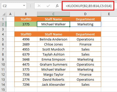
Here is an example of how to use Xlookup. In this case, I can enter a Staff ID into cell B2 which then performs an Xlookup on the Lookup_Value and returns the result for Staff Name and Department.
A noticeable difference in this data table is that my lookup values, being the staff ID’s, are not in ascending order which would not work if I was using Vlookup.

- Click in cell C2.
- Go to the Formulas tab and click the Lookup & References button.
- Select XLOOKUP from the list.
- Now use the mouse to select the Lookup_value which is the cell which contains the value you want to use to lookup information e.g. the Staff ID in cell B2.
- Click into the Lookup_array field and highlight where all the Staff ID values can be found E.g. B5 to B14.
- Now click in the Return_array field and select where all the values are located which contain the data you want to return back e.g. the Staff Names in cells C5 to C14.
- Click in the If_not_found field and enter a message if a staff ID cannot be found E.g. “Record not found“.
- By default the XLOOKUP will perform an exact match.
- Click OK.
- The name will be displayed for the corresponding Staff ID in cell B2.
- Enter a Staff ID in cell B2 which does not exist in the data. The If_not_found message you specified will appear.
Compatibility with other Excel versions
For the time being, Xlookup is only available to Microsoft 365 subscribers. If you are collaborating with other users within Excel who are using older versions of Excel, it may be safer to utilise the good-ole Vlookup or Hlookup.
Want to learn more?
If you are interested in upskilling yourself or your team to utilise the newest features of Microsoft Excel, or any Microsoft 365 product, be sure to check out our online or face to face course options.
Not sure which options would be suit your team? Contact us to discuss your needs and begin the process to undertake our free skills analysis.

